Build-Your-Own PyTorch Image Classifier via Transfer Learning
Thanks for taking an interest in my project! This originally started as an Image Classifier project I worked on in my Udacity Nanodegree program (highly recommended if you have the time & money!). In this notebook, I'll walk you through how the image classifier works. This does not explain how my command-line application works. This simply walks you through how the image classifier is trained and predicts. Please note...
- I am not a deep learning expert, nor do I claim to be. This notebook is a way for me to help me understand the concepts I'm learning.
- I am writing this under the assumption the reader has minimal knowledge of neural networks, but some knowledge of machine learning concepts.
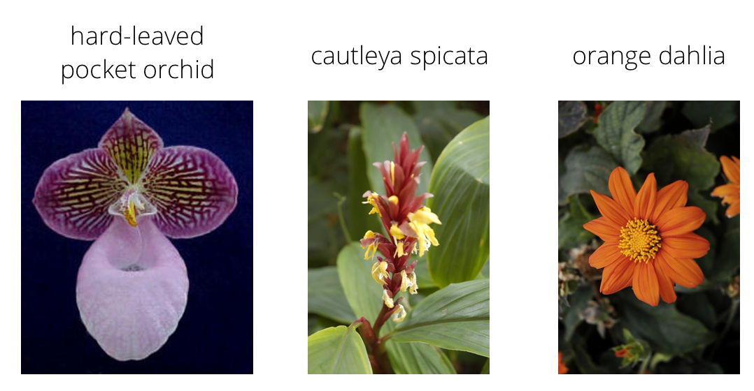
In this project, we will train an image classifier leveraging a pretraind Convolutional Neural Network using the PyTorch framework to recognize different species of flowers. You can imagine using something like this in a phone app that tells you the name of the flower your camera is looking at. In practice you'd train this classifier, then export it for use in your application. We'll be using this dataset of 102 flower categories, you can see a few examples below.
The project is broken down into multiple steps:
- Load and preprocess the image dataset
- Train the image classifier on your dataset
- Use the trained classifier to predict image content
Data Preparation
Importing Libraries
%matplotlib inline

import matplotlib.pyplot as plt
from PIL import Image

import numpy as np

import torch
from torch import nn, optim
import torch.nn.functional as F
from torchvision import datasets, transforms, models

from collections import OrderedDict
import time,json
from workspace_utils import active_session
Importing Data
In order for the neural network (BTW, whenever I say "model," I mean neural network) to train properly, our images need to be organized in folders named as their class name within training, testing, and validation folders. For example...
- train
- (Class Name to predict)
- (Image File)
- ...
- (Class Name to predict)
- ...
- (Class Name to predict)
- valid
- test
If your images aren't already organized like this, it can easily be done with a function like split folders.
data_dir = 'flowers'
train_dir = data_dir + '/train'
valid_dir = data_dir + '/valid'
test_dir = data_dir + '/test'
Tensor Data Prep
We're going to use pre-trained networks that come with the torchvision library. These networks were trained on the ImageNet dataset. All we have to do is replace the fully-connected classifier and re-train that on our flowers images. But in order for us to use the pretrained networks, we need the data to be prepared in a certain way, which we'll do in the cell below.
There are 3 general requirements that our image data need to meet in order to work with the pre-trained networks...
- Resized to 224x224 pixels
- In Tensor form
- In PyTorch, our data needs to be in the Tensor data type so we can load the images and pass it through our networks
- Tensors can be viewed as NumPy Arrays. This discussion is way over my head, but it explains the difference between matrices and tensors if you're interested. Otherwise, just think of tensors as an extension of matrices/arrays. Run the below code to see what I mean.
array = np.array([1,2,3])
tensor = torch.from_numpy(array)
print(tensor)
- Normalized to means [0.485, 0.456, 0.406] & standard deviations [0.229, 0.224, 0.225]
- To explain, image tensors in PyTorch have dimensions CxHxW (Color x Height x Width)
- Each pixel can be described as either one number (for grayscale) or 3 numbers (RedGreenBlue for colors)
- Each of these numbers need to be normalized to these means and standard deviations because this is how the ImageNet images were normalized. Otherwise, we'd be comparing apples to oranges.
- Each pixel can be described as either one number (for grayscale) or 3 numbers (RedGreenBlue for colors)
- To explain, image tensors in PyTorch have dimensions CxHxW (Color x Height x Width)
This 1) defines transformations for our data, 2) creates Torch Dataset objects using ImageFolder, and 3) creates DataLoader objects that lets us work with our data.
# Transformations literally "transform" our images into tensors that work with our model
# We want our training transformations to have some whacky randomness to it (i.e RandomHorizontalFlip)
    # This helps our model generalize to new images.
data_transforms_train = transforms.Compose([transforms.Resize(224),
                                        transforms.RandomHorizontalFlip(),
                                        transforms.RandomRotation(30),
                                        transforms.RandomResizedCrop(224),
                                        transforms.ToTensor(),
                                        transforms.Normalize([0.485, 0.456, 0.406],
                                                            [0.229, 0.224, 0.225])])

# We don't want to mess with the images we're using for validation,
    # so this is a more basic transform with no random mutations
data_transforms_test = transforms.Compose([transforms.Resize(224),
                                        transforms.CenterCrop(224),
                                        transforms.ToTensor(),
                                        transforms.Normalize([0.485, 0.456, 0.406],
                                                            [0.229, 0.224, 0.225])])

# Creating DataSet objects that "hold" our images
image_datasets_train = datasets.ImageFolder(train_dir,data_transforms_train)
image_datasets_valid = datasets.ImageFolder(valid_dir,data_transforms_test)
image_datasets_test = datasets.ImageFolder(test_dir,data_transforms_test)

# Creating DataLoader objects that let us work with our images in batches
train_dataloader = torch.utils.data.DataLoader(image_datasets_train,batch_size=64,shuffle=True)
valid_dataloader = torch.utils.data.DataLoader(image_datasets_valid,batch_size=64,shuffle=True)
test_dataloader = torch.utils.data.DataLoader(image_datasets_test,batch_size=64,shuffle=True)

# ImageFolder automatically maps the name of the image folders holding our data to the index that our model wil predict
    # If the first folder with images is "1", our model will predict "0" and we can use this mapping to map "0" to "1"
class_to_idx = image_datasets_train.class_to_idx
    # More on this later...
Label mapping
Our flower image folders aren't the actual names of the flowers. They're numbers instead. This json file has the mapping from flower names to folder labels. It was confusing for me to keep track of all the different labels when I worked on this project, but in sum, this is the flow...
1) Model predicts by giving us an index (the idx, between 0-101). 2) This idx corresponds to one of the folder labels (between 1-102) 3) The folder labels (between 1-102) correspond to flower names for which this json file helps us map.
file = 'cat_to_name.json'
with open(file, 'r') as f:
    cat_to_name = json.load(f)
no_output_categories = len(cat_to_name)
cat_to_name
Building & Training the Classifier
Below we will import one of the pre-trained networks from torchvision. We can leverage the model's convolutional layer weights and retrain the fully connected layers to classify our images. Below I've selected VGG16_bn (bn standing for batch normalization). VGG16_bn is a highly accurate Convolutional network, but is very slow to train.
Uploading the Pre-Trained Model & Preparing the Classifier
# Defining number of hidden units in our fully connected layer
hidden_units = 4096
# Downloading the pretrained model for us to use
model = models.vgg16_bn(pretrained=True)
# Freezing the feature parameters so they stay static (the convolutional layers)
    # Leveraging the feature parameters that were trained on ImageNet
for param in model.parameters():
    param.requires_grad = False
# This is the old classifier that came with vgg16_bn
model.classifier
# Defining the fully connected layer that will be trained on the flower images
classifier = nn.Sequential(OrderedDict([
                            ('fc1', nn.Linear(25088,hidden_units)),
                            ('relu', nn.ReLU()),
                            ('dropout', nn.Dropout(0.5)),
                            ('fc2', nn.Linear(hidden_units,no_output_categories)),
                            ('output', nn.LogSoftmax(dim=1))
                            ]))
model.classifier = classifier
model.classifier
Training & Testing the Network
If a GPU is available, we will use the GPU. The GPU (Graphical Processing Unit) was built to parallel process many matrix operations. This makes training a deep neural network VERY QUICK. Otherwise, the CPU will take forever (perhaps around 100x slower depending on the GPU). The cell below assigns the device variable to 'cuda' if we can use a GPU or to 'cpu' otherwise. We will move our model and our data over to the device of choice manually using...
model.to(device) or data.to(device).
device = torch.device("cuda:0" if torch.cuda.is_available() else "cpu")
Below is a heapload of code. Feel free to read through it if you want, but if you want the TL;DR version of this code, here it is...
- Sets hyperparameters for training (i.e. epochs, learning rate, etc).
- Uses active_session() (function provided by Udacity) to make sure the vm I used with GPU doesn't sleep on me while I'm training.
- Loops through epochs
- 1 batch is 64 images. The model trains on 20 batches at at time (as defined by
print_every) - After the 20 batches, we test our model's progress on the validation data
- Then we print our training and validation metrics (skip ahead below to see the metrics).
- 1 batch is 64 images. The model trains on 20 batches at at time (as defined by
model.to(device)

# Setting training hyperparameters
epochs = 10
optimizer = optim.Adam(model.classifier.parameters(),lr=.001)
criterion = nn.NLLLoss()
print_every = 20
running_loss = running_accuracy = 0
validation_losses, training_losses = [],[]

with active_session():
    for e in range(epochs):
        batches = 0
        # Turning on training mode
        model.train()
        for images,labels in train_dataloader:
            start = time.time()
            batches += 1
            # Moving images & labels to the GPU
            images,labels = images.to(device),labels.to(device)
            # Pushing batch through network, calculating loss & gradient, and updating weights
            log_ps = model.forward(images)
            loss = criterion(log_ps,labels)
            loss.backward()
            optimizer.step()
            # Calculating metrics
            ps = torch.exp(log_ps)
            top_ps, top_class = ps.topk(1,dim=1)
            matches = (top_class == labels.view(*top_class.shape)).type(torch.FloatTensor)
            accuracy = matches.mean()
            # Resetting optimizer gradient & tracking metrics
            optimizer.zero_grad()
            running_loss += loss.item()
            running_accuracy += accuracy.item()
            # Running the model on the validation set every 5 loops
            if batches%print_every == 0:
                end = time.time()
                training_time = end-start
                start = time.time()
                # Setting metrics
                validation_loss = 0
                validation_accuracy = 0
                # Turning on evaluation mode & turning off calculation of gradients
                model.eval()
                with torch.no_grad():
                    for images,labels in valid_dataloader:
                        images,labels = images.to(device),labels.to(device)
                        log_ps = model.forward(images)
                        loss = criterion(log_ps,labels)
                        ps = torch.exp(log_ps)
                        top_ps, top_class = ps.topk(1,dim=1)
                        matches = (top_class == \
                                   labels.view(*top_class.shape)).type(torch.FloatTensor)
                        accuracy = matches.mean()
                        # Tracking validation metrics
                        validation_loss += loss.item()
                        validation_accuracy += accuracy.item()

                # Tracking metrics
                end = time.time()
                validation_time = end-start
                validation_losses.append(running_loss/print_every)
                training_losses.append(validation_loss/len(valid_dataloader))

                # Printing Results
                print(f'Epoch {e+1}/{epochs} | Batch {batches}')
                print(f'Running Training Loss: {running_loss/print_every:.3f}')
                print(f'Running Training Accuracy: {running_accuracy/print_every*100:.2f}%')
                print(f'Validation Loss: {validation_loss/len(valid_dataloader):.3f}')
                print(f'Validation Accuracy: {validation_accuracy/ \
                                                len(valid_dataloader)*100:.2f}%')
                print(f'Training Time: {training_time:.3f} seconds for {print_every} batches.')
                print(f'Validation Time: {validation_time:.3f} seconds.\n')

                # Resetting metrics & turning on training mode
                running_loss = running_accuracy = 0
                model.train()
And just for fun, here's a plot of how our training and validation loss looked throughout training.
plt.figure()
plt.title("Training Summary")
plt.plot(training_losses,label='Training Loss')
plt.plot(validation_losses,label='Validation Loss')
plt.legend()
plt.show()

Testing The Network
We set aside testing data that our model has never seen to see how our trained model will perform.
test_accuracy = 0
for images,labels in test_dataloader:
    model.eval()
    images,labels = images.to(device),labels.to(device)
    log_ps = model.forward(images)
    ps = torch.exp(log_ps)
    top_ps,top_class = ps.topk(1,dim=1)
    matches = (top_class == labels.view(*top_class.shape)).type(torch.FloatTensor)
    accuracy = matches.mean()
    test_accuracy += accuracy
print(f'Model Test Accuracy: {test_accuracy/len(test_dataloader)*100:.2f}%')
The little guy did pretty well! Solid B-. Much better than I could do on flower images.
Saving Our Model
PyTorch allows us to save a "checkpoint" that essentially acts as a snapshot of our model. We need to save the state_dict in the checkpoint to do this. The state dict contains the learned weights that our model learned during training. So we can use our model to predict or test our model without having to train it again. Note that you can use this checkpoint to pause training and result later by saving your optimizer and scheduler (if learning decay was used) states as well.
# Setting destination directory to None saves the checkpoint in the current directory
dest_dir = None
def save_model(trained_model,hidden_units,output_units,dest_dir,model_arch,class_to_idx):
    '''
    This saves the model's state_dict, as well as a few other details that will help with loading the model for later use.
    '''
    model_checkpoint = {'model_arch':model_arch,
                    'clf_input':25088,
                    'clf_output':output_units,
                    'clf_hidden':hidden_units,
                    'state_dict':trained_model.state_dict(),
                    'model_class_to_idx':class_to_idx,
                    }
    if dest_dir:
        torch.save(model_checkpoint,dest_dir+"/"+model_arch+"_checkpoint.pth")
        print(f"{model_arch} successfully saved to {dest_dir}")
    else:
        torch.save(model_checkpoint,model_arch+"_checkpoint.pth")
        print(f"{model_arch} successfully saved to current directory as {model_arch}_checkpoint.pth")
save_model(model,hidden_units,no_output_categories,dest_dir,'vgg16_bn',class_to_idx)
Loading the Checkpoint
checkpoint = 'vgg16_bn_checkpoint.pth'
def load_checkpoint(filepath,device):
    '''
    Inputs...
        Filepath: location of checkpoint
        Device: "gpu" or "cpu"

    Returns:
        No. Input units, No. Output units, No. Hidden Units, State_Dict
    '''
    # Loading on GPU If available
    if device=="gpu":
        map_location=lambda device, loc: device.cuda()
    else:
        map_location='cpu'
    checkpoint = torch.load(f=filepath,map_location=map_location)
    return checkpoint['model_arch'],checkpoint['clf_input'], checkpoint['clf_output'], checkpoint['clf_hidden'],checkpoint['state_dict'],checkpoint['model_class_to_idx']
model_arch,input_units, output_units, hidden_units, state_dict, class_to_idx = load_checkpoint(checkpoint,device)
model.load_state_dict(state_dict)
Retesting Loaded Model
Just for fun :).
test_accuracy = 0
for images,labels in test_dataloader:
    model.eval()
    model.to(device)
    images,labels = images.to(device),labels.to(device)
    log_ps = model.forward(images)
    ps = torch.exp(log_ps)
    top_ps,top_class = ps.topk(1,dim=1)
    matches = (top_class == labels.view(*top_class.shape)).type(torch.FloatTensor)
    accuracy = matches.mean()
    test_accuracy += accuracy
    model.train()
print(f'Model Test Accuracy: {test_accuracy/len(test_dataloader)*100:.2f}%')
Inference/Prediction
Below we will use our model to predict/infer classes from whatever images we want.
Image Preprocessing
First step: preprocessing the images. Remember when we defined the data transformations for our training/testing data? We have to do the same thing on an image-by-image basis. We will use functions to preprocess our image and predict classes. That way, all we have to do to predict classes of images is to tell our functions where our image files are, and the data will be preprocessed and passed through our network easily.
We're using PIL to load images. Color channels of images are typically encoded as integers 0-255, but the model expected floats 0-1, normalized to specific means and standard deviations. We're going to convert the values to numpy arrays that we can work with and manipulate, then convert them to tensors that can be passed into our network.
# This is the location of the image file that we're going to work with
practice_img = './flowers/test/99/image_07833.jpg'
def process_image(image):
    '''
    Scales, crops, and normalizes a PIL image for a PyTorch model,

    Input: filepath to image

    Returns: NumPy Array of the image to be passed into the predict function
    '''
    # Open image
    im = Image.open(image).convert('RGB')
    # Resize keeping aspect ratio
    im.thumbnail(size=(256,256))
    # Get dimensions
    width, height = im.size
    # Set new dimensions for center crop
    new_width,new_height = 224,224
    left = (width - new_width)/2
    top = (height - new_height)/2
    right = (width + new_width)/2
    bottom = (height + new_height)/2
    im = im.crop((left, top, right, bottom))
    # Convert to tensor & normalize
    transf_tens = transforms.ToTensor()
    transf_norm = transforms.Normalize([0.485, 0.456, 0.406],[0.229, 0.224, 0.225])
    tensor = transf_norm(transf_tens(im))
    # Convert to numpy array
    np_im = np.array(tensor)
    return np_im
Udacity provided the imshow function below to help me check my work. This function converts a PyTorch tensor and displays it in the notebook. If my process_image function works, running the output through this function should return the original image (except for the cropped out portions).
def imshow(image, ax=None, title=None):
    """Imshow for Tensor."""
    if ax is None:
        fig, ax = plt.subplots()
        plt.tick_params(
            axis='both',
            which='both',
            bottom=False,
            top=False,
            left=False,
            labelbottom=False,
            labelleft=False,)
    # We need to move the color channel from the first dimension to the third dimension.
        # PyTorch expects color to be in the 1st dim, but PIL expects it to be in the 3rd!
    image = image.transpose((1, 2, 0))

    # Undo preprocessing
    mean = np.array([0.485, 0.456, 0.406])
    std = np.array([0.229, 0.224, 0.225])
    image = std * image + mean
    # Image needs to be clipped between 0 and 1 or it looks like noise when displayed
    image = np.clip(image, 0, 1)

    ax.imshow(image)

    return ax
Original Image...
im = Image.open(practice_img)
im

Preprocessing the image using process_image then undoing the preprocessing with imshow.
imshow(process_image(practice_img))

Class Prediction
Now we're going to use a function (class_to_label) that maps our label names to the folder names that our model was originally trained on. This is what the json file in the beginning is used for. Next we're going to write a predict function that will output our model's top-k predictions (in this example, we're having it predict the top 5 possible classes).
def class_to_label(file,classes):
    '''
    Takes a JSON file containing the mapping from class to label and converts it into a dict.
    '''
    with open(file, 'r') as f:
        class_mapping =  json.load(f)
    labels = []
    for c in classes:
        labels.append(class_mapping[c])
    return labels
# The ImageFolder dataset that we used for training in the very beginning has a class_to_idx attribute that
    # Helps us map our index predictions (0-101) to the folder labels (1-102).
        # Note we're using the class_to_label function in the cell above to map folder labels (1-102) to flower names
index_mapping = dict(map(reversed, class_to_idx.items()))
def predict(image_path, model,index_mapping, topk, device):
    ''' Predict the class (or classes) of an image using a trained deep learning model.
    - Mapping is the dictionary mapping indices to classes
    '''
    pre_processed_image = torch.from_numpy(process_image(image_path))
    pre_processed_image = torch.unsqueeze(pre_processed_image,0).to(device).float()
    model.to(device)
    model.eval()
    log_ps = model.forward(pre_processed_image)
    ps = torch.exp(log_ps)
    top_ps,top_idx = ps.topk(topk,dim=1)
    list_ps = top_ps.tolist()[0]
    list_idx = top_idx.tolist()[0]
    classes = []
    model.train()
    for x in list_idx:
        classes.append(index_mapping[x])
    return list_ps, classes
def print_predictions(probabilities, classes,image,category_names=None):
    '''
    Prints the system output of probabilities.
    '''
    print(image)
    if category_names:
        labels = class_to_label(category_names,classes)
        for i,(ps,ls,cs) in enumerate(zip(probabilities,labels,classes),1):
            print(f'{i}) {ps*100:.2f}% {ls.title()} | Class No. {cs}')
    else:
        for i,(ps,cs) in enumerate(zip(probabilities,classes),1):
            print(f'{i}) {ps*100:.2f}% Class No. {cs} ')
    print('')
probabilities,classes = predict(practice_img,model,index_mapping,5,device)
print_predictions(probabilities,classes,practice_img.split('/')[-1],file)
Sanity Checking
imshow(process_image(practice_img))
plt.figure()
plt.barh(class_to_label(file,classes),width=probabilities)
plt.title('Model Predictions')
plt.gca().invert_yaxis()
plt.show()

Conclusion
Thanks for taking the time to read through my notebook! Again, this doesn't go into the details on how my command-line application works. This explains the process of training a model and using it to predict classes of images. As you can see, Transfer Learning is a powerful thing. We successfully took a pre-trained Convolutional Neural Network, modified it, retrained it, and used it to predict species of 102 different flowers with over an 80% accuracy per testing results! The application train.py lets you repeat this process on ANY dataset you want given you have enough images to train on.
Cheers!